Getting Started with Sorting and Filtering

2.   All of the cells with data will now be selected. You can tell they are selected because they are highlighted in blue. 

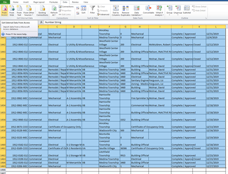
With your data selected, it is up to you what happens next.  If you go to the ribbon bar in Excel at the top of the screen, you can click on the “Data” tab. You could choose to either sort or filter. When you sort, it will ask what column you want to sort the list by. If you filter, it will give you those little drop-down lists in the header for the column where you can filter for blanks in the Use Type column.

1.  With the spreadsheet open, go to the Ribbon bar at the stop of the Excel screen and select " Insert."     NOTE: I recommend selecting the cell in the upper left of your data set (highlighted in yellow). It will help Excel automatically select your data for you.

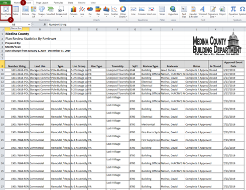
2.  Click on the button farthest to the left called “Pivot Table."

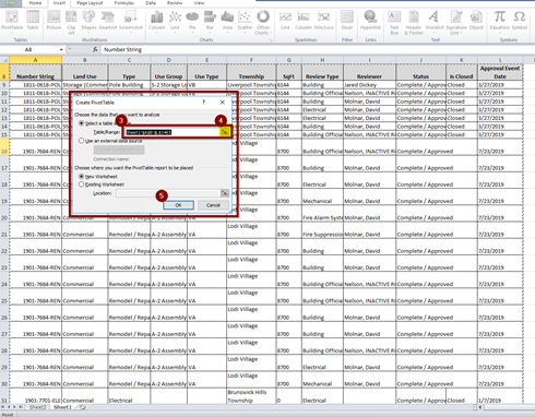
3.  A window will pop out and ask you what data to include in the pivot table. Because I selected that cell in the upper left, it picked up all the rows and columns I wanted to include.

4.  If the data selected does not match what you want, you can click and drag to the select the data you want included.

5.  Click OK.

6.  A new sheet will be inserted and will automatically be named Sheet 2. The sheet will look mostly blank if you click in a cell outside the Pivot Table box (outside area marked with X). Click in the Pivot Table Area to get the list of choices to appear in the upper right.

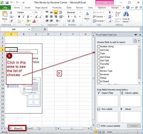
7.  Check the boxes of the data you want to summarize. I checked “Number String," then "Use Type,” and “Township." I chose these because I wanted to know how many reviews were performed for each Township and split them out by use Type Category. I chose Number String because the table needs something to count. 

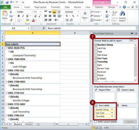
A Number String has letters and numbers in it (so my Pivot Table will default to counting it), and is never blank in my data set (so the total count will always be the same as the number of rows). 

(If I chose a field that only had numbers in it, Excel would automatically try to Sum instead of Count.)

8.  The boxes I checked show up in the row labels box by default. Right now, the table doesn’t look like what I showed you, but don’t fret. It will in the next steps.

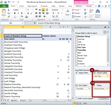
9.  I left “Township” in the Row Label box because I wanted a list of townships to appear on the left of the Pivot Table. I dragged “Use Type” to the Column Labels box because it wants columns for each use type to appear across the top.

10.  I dragged “Number String” to the Values box because (as mentioned in #7) I wanted the table to count how many.

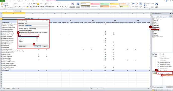
11.   I decided I wanted to also now the square footage of the construction that was reviewed. So, I checked the "SqFt" box.

12.   SqFt initially showed up in the Row Label box, but I wanted to total the square footage. So, I dragged it to the Values box.

13.   Excel counted my square footage instead of adding it all together. To change this, I clicked on “Count of SqFt” and chose the “Value Field Settings” option.

14.   A new window popped out, and I selected Sum instead of Count so I could get the total square footage by Use Type for each Township.

15.  When you click OK, the table will update.